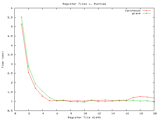
First Graph: My first graph. I'm mapping the depth of the ILP
for two 64-bit Linux computers in the CS Department. I made this in gnuplot!
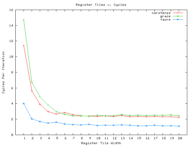
Second Graph: I added Faure, a solaris machine, to the graph!
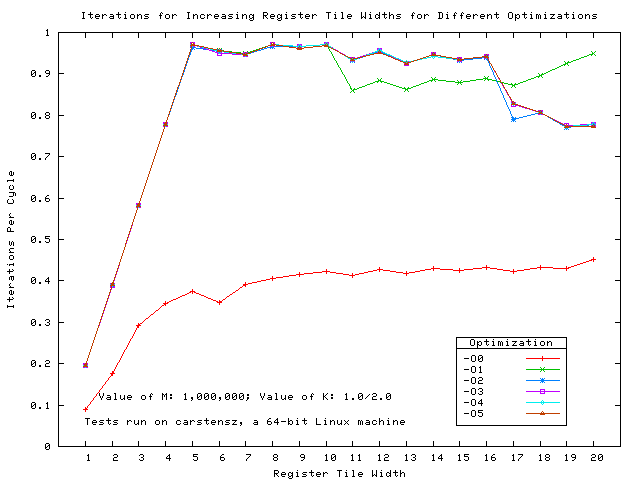
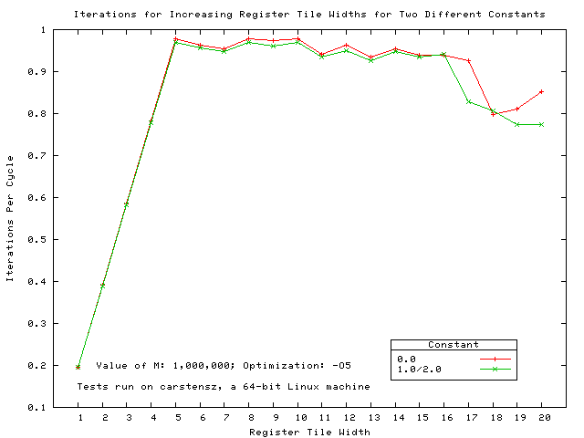
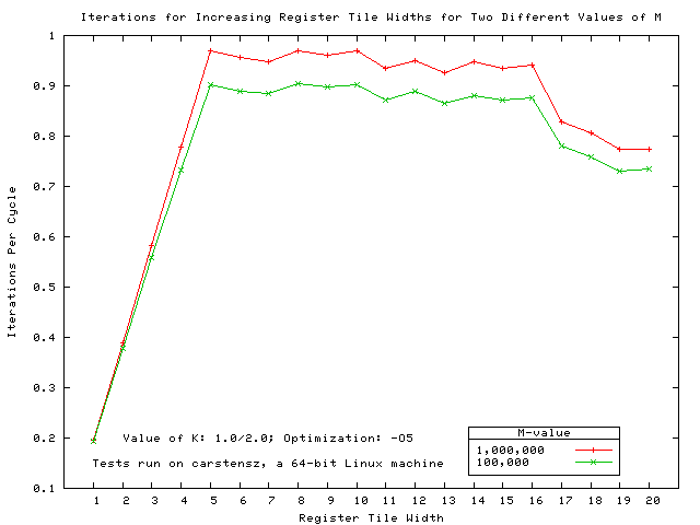
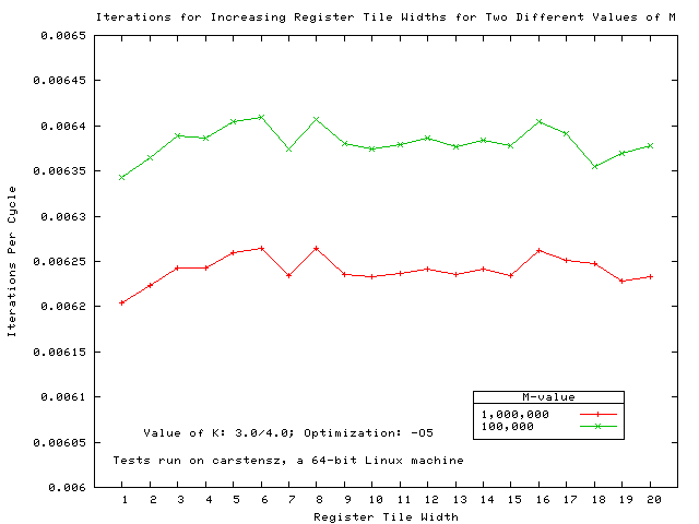
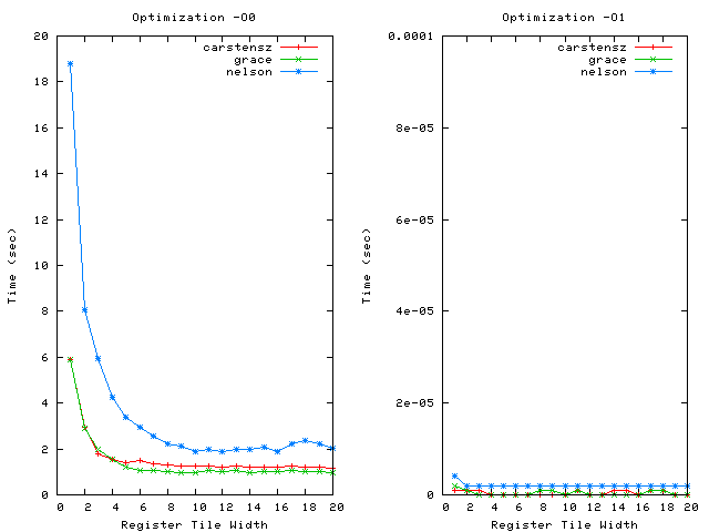
Graphs for carstensz: After running programs with several variables, I made a few
graphs. These were all run on my computer, carstensz.
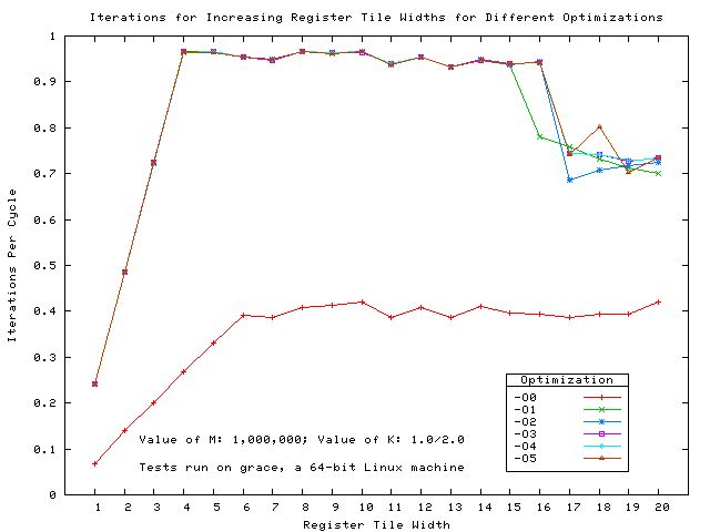
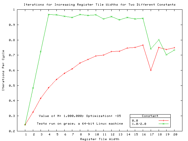
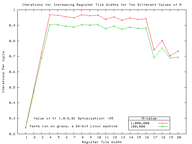
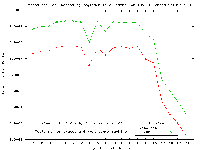
Graphs for grace: I also made a set of graphs for grace, another 64-bit Linux machine.
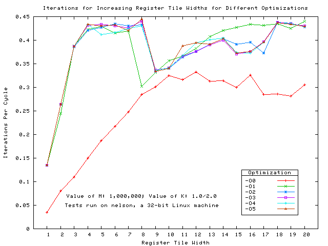
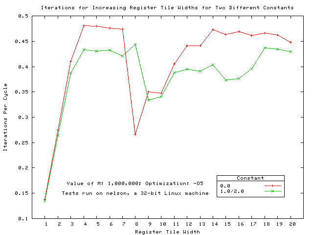
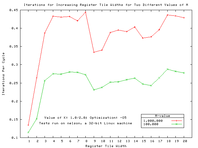
Graphs for nelson: And here are the graphs for nelson, a 32-bit Linux machine.
Comparison graphs: Here are a couple of graphs I made with comparisons across the computers.
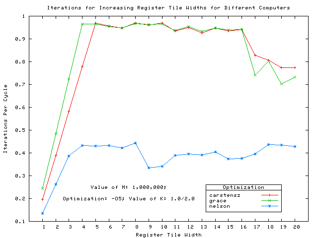
Conclusions: Based on these preliminary graphs, I've been able to come to a few conclusions:
- A constant of 1 gets optimized away in everything greater than -O0, and consequently cannot be used in comparisons.
- A constant of 0.75 is very costly for the compiler and does not appear to be affected by register tile size (why?)
- Constants of 0 and of 0.5 are approximately equal in efficiency, and benefit from register tile size. By looking at either of these constants at optimizations greater than -O0 there is a clear "peak" in computation efficiency; this is the maximum amount of ILP for a particular computer.
- For grace, the efficiency peaks at register tiles of size 4
- For carstensz, the efficiency peaks at register tiles of size 5
- For nelson, the efficiency peaks at register tiles of size 4